library("tidyverse")

pog_cts <- read_rds("data-derived/pog_cts.rds")3 Plot probabilities
In the last chapter, we completed data preprocessing and saved the resulting data to as an R binary RDS file, pog_cts.rds. In this chapter, we will import the data and use it to recreate some of the figures in Weighall et al. (2017).
First, let’s load in {tidyverse} and then import the point-of-gaze data.
As usual, the first thing we should do is have a look at our data.
# A tibble: 1,021,288 × 5
   sub_id  t_id   f_c role   pad
    <int> <int> <int> <fct>  <lgl>
 1      1     1   -90 target FALSE
 2      1     1   -89 target FALSE
 3      1     1   -88 target FALSE
 4      1     1   -87 target FALSE
 5      1     1   -86 target FALSE
 6      1     1   -85 target FALSE
 7      1     1   -84 target FALSE
 8      1     1   -83 target FALSE
 9      1     1   -82 target FALSE
10      1     1   -81 target FALSE
# … with 1,021,278 more rows
The data has sub_id and t_id which identify individual subjects and trials-within-subjects, respectively. But we are missing iformation about what group the subject belongs to (adult or child) and what experimental condition each trial belongs to.
3.1 Merge eye data with information about group and condition
3.1.1 Activity: Get trial condition
The first step is to create trial_cond, which has information about the group that each subject belongs to, the competitor type (existing or novel), and the condition (the identity of the critical object). The information we need is distributed across the subjects, trials, and stimuli tables (see Appendix A). Create trial_cond so that the resulting table matches the format below.
# A tibble: 5,644 × 5
   sub_id group  t_id ctype crit
    <int> <chr> <int> <chr> <chr>
 1      1 adult     1 novel competitor-day2
 2      1 adult     2 novel competitor-day1
 3      1 adult     3 exist competitor
 4      1 adult     4 exist competitor
 5      1 adult     6 novel untrained
 6      1 adult     7 novel competitor-day1
 7      1 adult    11 novel untrained
 8      1 adult    13 novel competitor-day2
 9      1 adult    14 novel untrained
10      1 adult    16 novel untrained
# … with 5,634 more rows
Solution
trials <- read_csv("data-raw/trials.csv",
                   col_types = "iiiiii")

stimuli <- read_csv("data-raw/stimuli.csv",
                    col_types = "iiciccc")

subjects <- read_csv("data-raw/subjects.csv",
                     col_types = "ic")

trial_cond <- trials %>%
  inner_join(stimuli, "iv_id") %>%
  inner_join(subjects, "sub_id") %>%
  select(sub_id, group, t_id, ctype, crit)
3.2 Plot probabilities for existing competitors
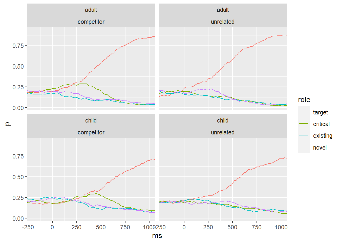
We want to determine the probability of looking at each image type at each frame in each condition. We will do this first for the existing competitors. Note there were two conditions here, indexed by crit: competitor and unrelated, corresponding to whether the critical image was a competitor or an unrelated item.
3.2.1 Activity: Probs for exist condition
From trial_cond, include only those trials where ctype takes on the value exist, combine with pog_cts, and then count the number of frames in each region for every combination of the levels of group (adult, child) and crit (competitor, unrelated). The resulting table should have the format below, where Y is the number of frames for each combination. While you’re at it, convert f_c to milliseconds (1000 * f_c / 60). Call the resulting table count_exist.
Hint: Counting things
Use the count() function from {dplyr}. Take note of the .drop argument to deal with possible situations where there are zero observations. For example:
pets <- tibble(animal = factor(rep(c("dog", "cat", "ferret"), c(3, 2, 0)),
                               levels = c("dog", "cat", "ferret")))

pets
# A tibble: 5 × 1
animal
<fct>
1 dog
2 dog
3 dog
4 cat
5 cat pets %>%
count(animal)# A tibble: 2 × 2
animal n
<fct> <int>
1 dog 3
2 cat 2pets %>%
count(animal, .drop = FALSE)# A tibble: 3 × 2
animal n
<fct> <int>
1 dog 3
2 cat 2
3 ferret 0# A tibble: 3,620 × 6
group crit f_c role Y ms
<chr> <chr> <int> <fct> <int> <dbl>
1 adult competitor -90 target 54 -1500
2 adult competitor -90 critical 55 -1500
3 adult competitor -90 existing 55 -1500
4 adult competitor -90 novel 75 -1500
5 adult competitor -90 (blank) 181 -1500
6 adult competitor -89 target 59 -1483.
7 adult competitor -89 critical 60 -1483.
8 adult competitor -89 existing 58 -1483.
9 adult competitor -89 novel 74 -1483.
10 adult competitor -89 (blank) 169 -1483.
# … with 3,610 more rows
Solution
count_exist <- trial_cond %>%
  filter(ctype == "exist") %>%
  inner_join(pog_cts, c("sub_id", "t_id")) %>%
  count(group, crit, f_c, role, name = "Y", .drop = FALSE) %>%
  mutate(ms = 1000 * f_c / 60)
To calculate the probability for each value of role, we need to calculate the number of opportunities for each combination of group, crit, and f_c, storing this in N. We do this using a windowed mutate, grouping the data before adding N for each group. We can then calculate the probability as p = Y / N.
prob_exist <- count_exist %>%
  group_by(group, crit, f_c) %>%
  mutate(N = sum(Y), p = Y / N) %>%
  ungroup()
Now we are ready to plot.
ggplot(prob_exist %>% filter(role != "(blank)"),
       aes(ms, p, color = role)) +
  geom_line() +
  facet_wrap(group ~ crit, nrow = 2)  +
  coord_cartesian(xlim = c(-200, 1000))