Linear Mixed-Effects Models
Dale Barr
University of Glasgow
Overview
- introduction to linear mixed-effects modeling
- example: sleepstudy data
- distinguish complete pooling, no pooling and partial pooling approaches
- understand the DGP behind multi-level data and estimation with
lme4::lmer()
Multilevel data
- All parametric models assume model residuals are IID (“independently and identically distributed”)
- Data often has ‘clusters’ of correlated observations due to
- natural clustering
- multistage sampling
pros and cons of LMEMs
Pros
- powerful and expressive
- modeling of continuous & categorical predictors
- unbalanced/missing data (partial pooling)
- multiple random factors
- discrete DVs and/or non-normal distributions
Cons
- complex
- estimated iteratively and may not converge!
Understanding multi-level modeling
Belenky et al. (2003)
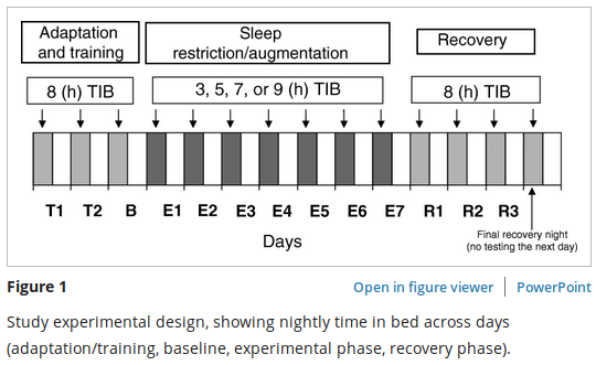
Worked example: Belenky et al. (2003) sleepstudy data
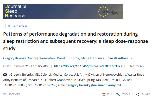
Belenky et al. (2003)
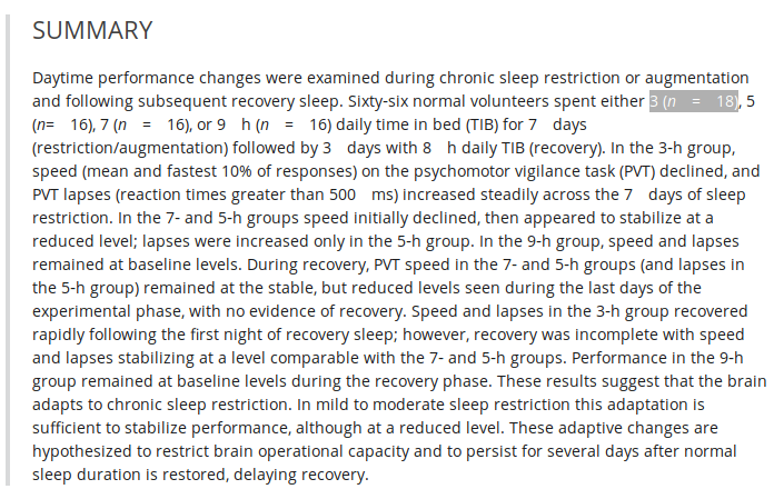
Belenky et al. (2003)
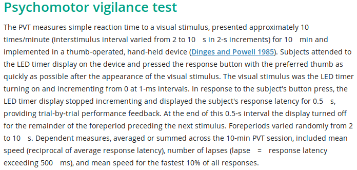
Psychomotor vigilance test
lme4::sleepstudy
\(Y_{ij} = \beta_0 + \beta_1 X_{ij} + e_{ij}\)
but: observations within subject not independent
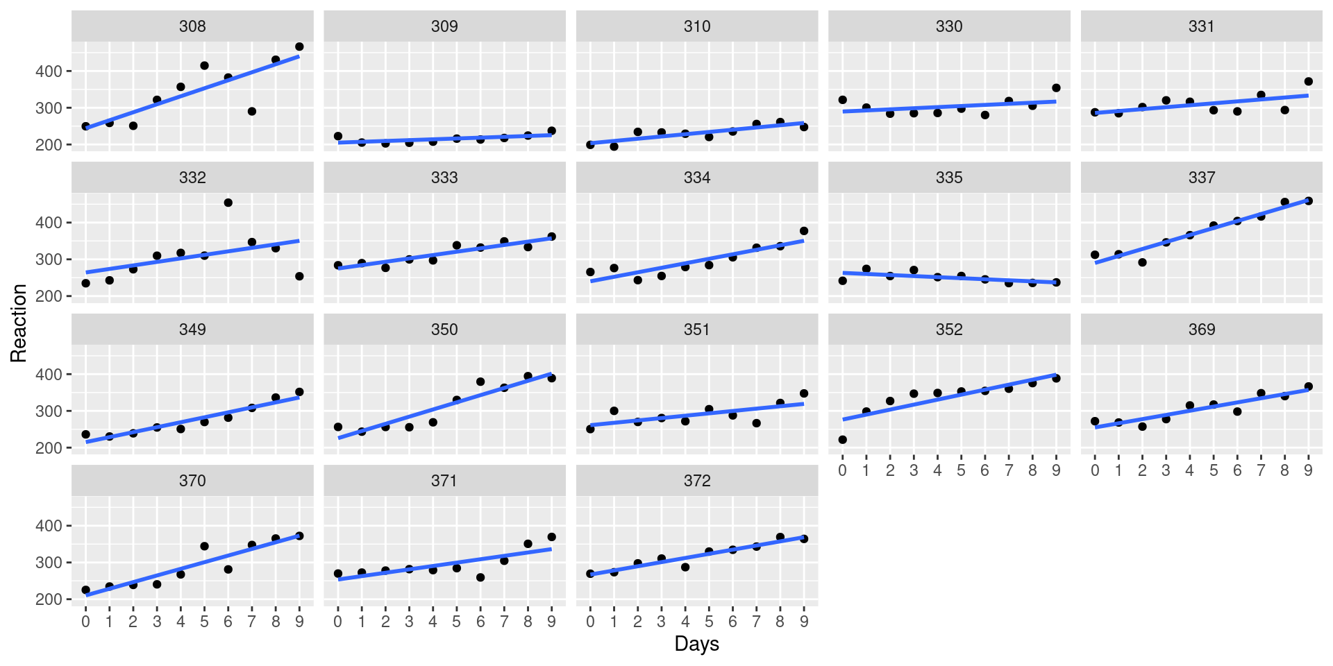
Approaches to ML data
- complete pooling
- ignore dependencies in the data
- no pooling
- account for dependencies by fitting each subject independently
- partial pooling
- account for dependencies by explicitly modeling them
- fit for each subject informed by the fits for other subjects
DGP and estimation
GLM for sleepstudy
Level 1:
\[Y_{ij} = \beta_0 + \beta_1 X_{ij} + e_{ij}\]
Level 2:
\[\beta_0 = \gamma_{00} + S_{0i}\]
\[\beta_1 = \gamma_{10} + S_{1i}\]
Variance Components
\[\left< S_{0i}, S_{1i} \right> \sim N(\left< 0, 0 \right>, \mathbf{\Sigma})\]
\[\mathbf \Sigma = \left( \begin{array}{cc} {\tau_{00}}^2 & \rho\tau_{00}\tau_{11} \\ \rho\tau_{00}\tau_{11} & {\tau_{11}}^2 \\ \end{array} \right)\]
\[e_{ij} \sim N(0, \sigma^2)\]
Estimation
Linear mixed model fit by REML ['lmerMod']
Formula: Reaction ~ Days + (Days | Subject)
   Data: sleepstudy

REML criterion at convergence: 1743.6

Scaled residuals:
    Min      1Q  Median      3Q     Max
-3.9536 -0.4634  0.0231  0.4634  5.1793

Random effects:
 Groups   Name        Variance Std.Dev. Corr
 Subject  (Intercept) 612.10   24.741
          Days         35.07    5.922   0.07
 Residual             654.94   25.592
Number of obs: 180, groups:  Subject, 18

Fixed effects:
            Estimate Std. Error t value
(Intercept)  251.405      6.825  36.838
Days          10.467      1.546   6.771

Correlation of Fixed Effects:
     (Intr)
Days -0.138
model syntax
DV ~ iv1 + iv2 + (iv1 | random_factor)
lmer(Reaction ~ Days + (1 | Subject), sleepstudy) # (1) random intercept

lmer(Reaction ~ Days + (1 + Days | Subject), sleepstudy) # (2) random slope model.
lmer(Reaction ~ Days + (Days | Subject), sleepstudy) # (3) identical to (2)

lmer(Reaction ~ Days + (1 | Subject) + (0 + Days | Subject)) # (4) zero-covariances
lmer(Reaction ~ Days + (Days || Subject), sleepstudy) # (5) identical to (4)
p-values: model comparison
# A tibble: 2 × 8
   npar   AIC   BIC logLik deviance Chisq    Df `Pr(>Chisq)`
  <dbl> <dbl> <dbl>  <dbl>    <dbl> <dbl> <dbl>        <dbl>
1     5 1785. 1801.  -888.    1775.  NA      NA  NA
2 6 1764. 1783. -876. 1752. 23.5 1 0.00000123p-values: t-as-z
 (Intercept)         Days
0.000000e+00 3.218759e-12