Statistical Models

Dale Barr

University of Glasgow

Statistical (& “Scientific”) Models

Semester One: How do I translate a study design into a statistical model for analysis?
Semester Two: How do I develop an idea and translate it into a study design?

The approach

We want our analyses to be:

reproducible
transparent
generalizable
flexible

Recipes encourage poor practice

“If all you have is a hammer, everything looks like a nail”

violation of assumptions
- especially: independence
discretization of predictors
treating categorical data as continuous
over-aggregation
mindless statistics

What do they have in common?

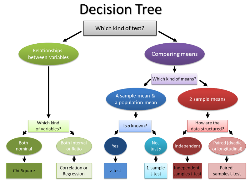
t-test
correlation & regression
multiple regression
analysis of variance
mixed-effects modeling

All are special cases of the General Linear Model (GLM).

GLM approach

Define a mathematical model representing the processes that are assumed to give rise to the data
Estimate the parameters of the model
Validate the model
Transparently report what you did
- share your code
- anonymize and share your data (ethics permitting)

Models are just… models

A statistical model is a simplification and idealization of reality that captures our key assumptions about the processes underlying data (the data generating process or DGP).

Importance of data simulation

Data simulation is a litmus test of understanding a statistical approach.
- Can you generate simulated data that would meet the assumptions of the approach?
  - If not, you don’t understand it (yet!)
Being able to specify the DGP is key to study planning (power)

Example: Parent reflexes

Does being the parent of a toddler sharpen your reflexes?

simple response time to a flashing light
dependent (response) variable: mean RT for each parent

Simulating data

set.seed(2021) # RNG seed: arbitrary integer value
parents <- rnorm(n = 50, mean = 480, sd = 40)

parents

 [1] 475.1016 502.0983 493.9460 494.3853 515.9221 403.0972 490.4698 516.6227
 [9] 480.5509 549.1985 436.7118 469.0870 487.2798 540.3417 544.1788 406.3410
[17] 544.9324 485.2556 539.2449 540.5327 442.3023 472.5726 435.9550 528.3246
[25] 415.0025 484.2151 421.7823 465.8394 476.2520 524.0267 401.4470 422.0822
[33] 520.7777 423.1433 455.8187 416.6610 428.5627 421.8126 476.5172 500.1895
[41] 484.6555 550.4085 466.1953 564.8000 478.6249 448.3138 539.0206 450.9777
[49] 492.4952 507.6786

Control group

set.seed(2021) # RNG seed: arbitrary integer value
parents <- rnorm(n = 50, mean = 480, sd = 40)

parents

 [1] 475.1016 502.0983 493.9460 494.3853 515.9221 403.0972 490.4698 516.6227
 [9] 480.5509 549.1985 436.7118 469.0870 487.2798 540.3417 544.1788 406.3410
[17] 544.9324 485.2556 539.2449 540.5327 442.3023 472.5726 435.9550 528.3246
[25] 415.0025 484.2151 421.7823 465.8394 476.2520 524.0267 401.4470 422.0822
[33] 520.7777 423.1433 455.8187 416.6610 428.5627 421.8126 476.5172 500.1895
[41] 484.6555 550.4085 466.1953 564.8000 478.6249 448.3138 539.0206 450.9777
[49] 492.4952 507.6786

control <- rnorm(n = 50, mean = 500, sd = 40)

control

 [1] 479.9884 409.7652 501.7497 485.2473 461.5911 504.1507 517.0916 493.1807
 [9] 438.0344 439.7760 500.6417 492.5854 515.6773 469.7316 509.2567 460.6555
[17] 522.6032 564.6701 489.9214 457.7649 486.0707 498.2804 444.0978 559.6087
[25] 458.4245 490.5222 460.0343 444.2983 539.2802 514.4376 486.4996 474.2645
[33] 413.3246 525.3316 494.2034 450.3989 521.3584 436.4694 460.3614 519.3304
[41] 532.4247 488.2534 497.8617 529.4074 500.5994 495.1199 474.1291 465.2857
[49] 479.6520 416.8966

\(t\)-test

t.test(parents, control, var.equal = TRUE)


    Two Sample t-test

data:  parents and control
t = -0.5871, df = 98, p-value = 0.5585
alternative hypothesis: true difference in means is not equal to 0
95 percent confidence interval:
 -20.89804  11.35576
sample estimates:
mean of x mean of y 
 480.6351  485.4062

Analysis of variance (ANOVA)

dat <- tibble(
  group = rep(c("parent", "control"), 
              c(length(parents), length(control))),
  rt = c(parents, control))

dat

# A tibble: 100 × 2
   group     rt
   <chr>  <dbl>
 1 parent  475.
 2 parent  502.
 3 parent  494.
 4 parent  494.
 5 parent  516.
 6 parent  403.
 7 parent  490.
 8 parent  517.
 9 parent  481.
10 parent  549.
# ℹ 90 more rows

summary(aov(rt ~ group, dat))

            Df Sum Sq Mean Sq F value Pr(>F)
group        1    569   569.1   0.345  0.558
Residuals   98 161801  1651.0

Regression

\[Y_i = \beta_0 + \beta_1 X_i + e_i\]

\[e_i \sim N(0, \sigma^2)\]

summary(lm(rt ~ group, dat))


Call:
lm(formula = rt ~ group, data = dat)

Residuals:
    Min      1Q  Median      3Q     Max 
-79.188 -27.147   3.214  29.341  84.165 

Coefficients:
            Estimate Std. Error t value Pr(>|t|)    
(Intercept)  485.406      5.746  84.472   <2e-16 ***
groupparent   -4.771      8.127  -0.587    0.558    
---
Signif. codes:  0 '***' 0.001 '**' 0.01 '*' 0.05 '.' 0.1 ' ' 1

Residual standard error: 40.63 on 98 degrees of freedom
Multiple R-squared:  0.003505,  Adjusted R-squared:  -0.006663 
F-statistic: 0.3447 on 1 and 98 DF,  p-value: 0.5585

Single- vs Multi-level data

sub	A	Y
1	A1	774
2	A1	845
3	A1	786
4	A2	751
5	A2	680
6	A2	805

sub	stim	A	Y
1	A	A1	787
1	B	A1	530
1	C	A1	743
2	A	A2	859
2	B	A2	849
2	C	A2	787

Issues with multi-level data

GLMs assume independence of residuals
Observations within a cluster (unit) are not independent
Any sources of non-independence must be modeled (we’ll learn this later!) or aggregated away
Typical consequence of failing to do so: High false positives

Regression: Killer App

technique	t-test	ANOVA	regression
Categorical IVs	✓	✓	✓
Continuous DVs	✓	✓	✓
Continuous IVs		-	✓
Multi-level data	-	-	✓
Categorical DVs			✓
Unbalanced data	-	-	✓
>1 sampling unit			✓

Four functions to rule them all

Is the data single- or multi-level?
Is the response continuous or discrete?
How are the observations distributed?

structure	response	distribution	R function
single	cont	normal	`base::lm()`
single	cont/disc	various	`base::glm()`
multi	cont	normal	`lme4::lmer()`
multi	cont/disc	various	`lme4::glmer()`